nLab identity type
Context
Equality and Equivalence
-
equality (definitional, propositional, computational, judgemental, extensional, intensional, decidable)
-
isomorphism, weak equivalence, homotopy equivalence, weak homotopy equivalence, equivalence in an (∞,1)-category
-
Examples.
Type theory
natural deduction metalanguage, practical foundations
type theory (dependent, intensional, observational type theory, homotopy type theory)
computational trinitarianism =
propositions as types +programs as proofs +relation type theory/category theory
Induction
Rules
Categorical semantics
Examples
Contents
- Idea
- Definition in Martin-Löf type theory
- With inference rules
- Induction using functions instead of type families
- In terms of inductive types
- -conversion and the reflection rule
- Dependent universal property
- Variants of the identity type
- Definition from an interval type
- Definition in observational type theory
- Definition in cubical type theory
- Categorical semantics
- Related concepts
- References
Idea
In type theory – where one understands every piece of data (every “term”) as being of a given type which specifies its operational behaviour – identity types (maybe better: identification types) are the types of those terms which serve as “witnesses” or “certificates” (see at “propositions as types”) of identification of terms of type .
What exactly this means depends on the nature of the ambient type theory and the choices for the inference rules of the identity types (see at extensional and intensional type theory). In some setups (see below), having a term of identity type means much the same as having an equality in classical mathematics, and for this (historical) reason identity types are often denoted simply by equality signs, for better or worse.
But the power of the notion of identity types goes beyond this classical situation and results from the fact that they may give the notion of equality a constructive meaning (“propositional equality”). Taking this constructive principle of identity types to its logical conclusion, leads – notably in Martin-Löf dependent type theory, see below – to identity types which themselves have identity types, reflecting identifications-of-identification, and so on, paralleling the higher structure of homotopies and homotopies of homotopies in homotopy theory, whence one refers to type theories with such identity types also as homotopy type theories.
Note on terminology
There are many different names used for this particular dependent type, as well as many different names used for the terms of this dependent type. These include the following:
| name of type | name of terms |
|---|---|
| identity type | identities |
| path type | paths |
| identification type | identifications |
| equality type | equalities |
These four names have different reasons behind the use of the name:
-
The name “identity type” comes from the fact that the identity type is the canonical one-to-one correspondence of the identity equivalence on a type , as well as philosophically that it represents the notion of “identity” of an object; see identity of indiscernibles.
-
The name “path type” comes from either the fact that the identity type is a path space object in the categorical semantics, or that every term in the identity type is represented by a function from the interval type, just as paths in topology are represented by a function from the unit interval.
-
The name “identification type” comes from the fact that elements represents identification certificates in computing, as well as philosophically that it represents the notion of “identifying” two objects together.
-
The name “equality type” comes from the fact that it is the typal equivalent of propositional equality from first order logic with equality.
ML identity types
The inference rules for identity types in Martin-Löf-/homotopy type theory (ML identity types) may be understood as follows (exposition and diagrams follow Myers et al. 2023):
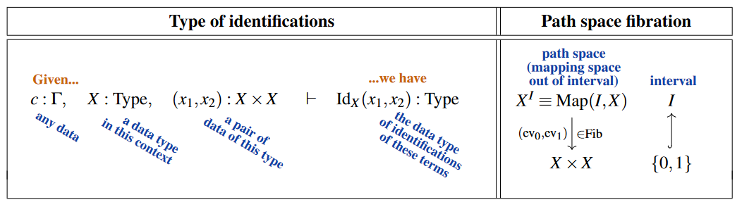
(0) – There is a notion of identification. To start with, for every type and any pair of its terms, let’s denote the type of identifications of with by (other common notation for identity types is “” which, when adopted, requires authors to make up new symbols, like , for actual equalities). In the jargon of dependent type theory this means that there is a type formation rule for identity types as shown on the left here:
Beware that in type theory generally and specifically in this entry further below, the self-identification certificate is often denoted “”, alluding to reflexivity of an equality relation.
On the right we are indicating, here and in the following, the categorical semantics of the judgement on the left, under the relation between type theory and category theory, specifically between dependent type theory and LCC category theory. The lay reader may take the diagrams shown on the right as intuitive illustrations of dependent types as bundles of types, their terms as sections, etc. Technically, these are diagrams in some locally cartesian closed (model) category. (Beware that we are showing an actual interval object for ease of illustration, but its existence is not required by the rules for ML identity types: may denote an object that does not arise as an internal hom. Making the interval object syntactically explicit leads to “cubical identity types”, see below.)
The archetypical example is the (classical model structure on) SimplicialSets (with interval object the 1-simplex) in which case all fibrations shown are Kan fibrations between Kan complexes which may be thought of as models for (fibrations of) -groupoids. But the power of ML identity types is that they may just as well be interpreted in much more general model categories, such as the injective model structure on simplicial presheaves over any simplicial site, modelling -toposes of -stacks.
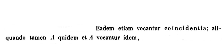
Now to consider three “self-evident” properties of the notion of identifications (Latin quotes from Gottfried Leibniz 1700, p. 228 and p. 230 in Gerhard 1890), expressed in type theoretic language:
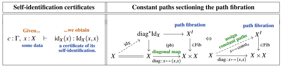
(I) – All data is identified with itself.
This “first law of thought” is the term introduction-rule for identity types:
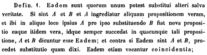
(IIa) – Substitution of identifications preserves computations. This is Leibniz’s “salva veritate”-principle phrased operationally/constructively:
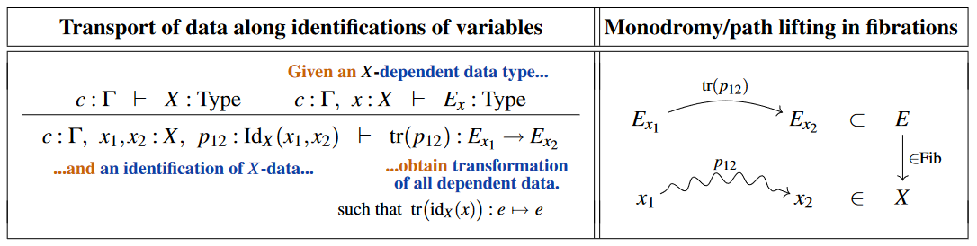
In homotopy type theory this has come to be known as transport, compatible with the fact that its categorical semantics is that of path lifting in Kan fibrations, which in the case of discrete fibrations (covering spaces) underlying flat principal bundles or flat vector bundles (“local systems”) is the parallel transport/holonomy/monodromy of the corresponding flat connection.

(IIb) – An identification identifies itself with a self-identification. While one may argue that this is still “self-evident”, it is more subtle than the previous two principles. In particular, it concerns an identification of identifications, a possibility that was ignored by the logical forefathers (Leibniz highlights at least the composition of identifications, such as ).
In type theory language, the existence of these identifications-of-identifications is the following judgement (with denoting the dependent sum-type):
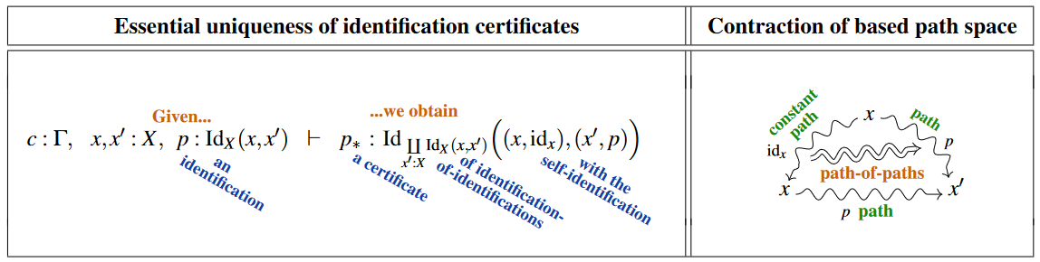
(An intuitive categorical semantics is schematically indicated on the right, with the certificate pictured as a copy of on the bottom together with a “path-of-paths” relating the concatenated path to . This is valid when realized in the model structure on simplicial sets or any model structure on simplicial presheaves, literally given by triangular diagrams as above, these being 1-simplices in when hom-adjointly regarded as 2-simplices in . However, this is not literally what the principle says when expressed in type theory, where there is no concatenated path — although after we have identity types with all of their rules, it can be proved equivalent.)
(J) (II) – Id-induction. Applying the above transport rule (IIa) to the identifications-of-identifications provided by the composition rule (IIb) yields the following “J-rule”, which was not known to the forefathers:
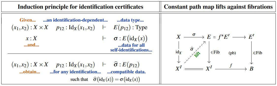
(This “induction-rule” for identity types was proposed in Martin-Löf 1975, §1.7 and p. 94; its modern rendering as a formal inference rule is due to Nordström, Petersson & Smith 1990, §8.1. It may be understood as the term elimination rule (see below) or the induction-principle (see further below) for identity types, whence also called “Id-elimination” or “Id-induction”, or similar.)
While the J-rule is naturally understood as the application of the transport rule (IIa) to the identifications-of-identification provided by the composition rule (IIb), it also implies both these rules, hence is equivalent to their combination (IIa and IIb). (This fact was briefly mentioned by Coquand 2011, slides 26+28 and amplified by Ladyman & Presnell 2015; the detailed proof is spelled out by Götz 2018, §4.2.)
Importantly, as indicated on the right above, the categorical semantics of the J-rule is manifestly that of the left lifting property of against all fibrations, which means that this rule manifestly prescribes the interpretation of identity types by “very good path space objects ” in the sense of model category theory (cf. Shulman 2012 III, Slide 34; Riehl 2022, §1.1). It is this fact which connects ML identity types to the notion of homotopy in homotopy theory, hence to the interpretation of Martin-Löf dependent type theory as “homotopy type theory” with categorical semantics in locally cartesian closed -categories.
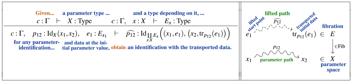
Incidentally, another immediate consequence of the J-rule is the following refinement of the transport rule (IIa), which is closer to what Leibniz may have recognized:
(IIa’) – Substitution of identifications preserves identifications.
Cubical identity types
Besides the Martin-Löf identity types above there are other version of identity types considered in the literature, notably there are variants which share the homotopy-theoretic interpretation but differ in some technical details:
For instance, cubical identity types (such as Swan identity types) are the identity types in cubical type theory, which are such that that applied to the type universe they provably (computationally) satisfy the univalence axiom.
Namely, the J-rule in Martin-Löf dependent type theory above still involves an ordinary judgmental equality in its statement that the lifted term is equal to the given term after restriction to self-identitfication. Cubical identity types essentially turns this equality itself into a typal equality.
Similarly, higher observational type theory has its appropriate version of higher identity types.
Notice that higher identity types restricted specifically to h-sets behave again more like ordinary equality does (by definition of h-set).
More specifically, there are also strict identity types, strictly without an homotopy-theoretic interpretation:
Strict identity types
Since there are two notions of equality in type theory, there are similarly two notions of the J-rule in type theory. The judgmental J-rule states that is judgmentally equal to (i.e. ). This is in contrast to the typal J-rule above, which states that there is a dependent term
Identity types which satisfy the judgmental J-rule can be called strict identity types, while identity types which only satisfy the typal J-rule can be called weak identity types, in parallel with similar definitions for a (weak and strict) Tarski universe. Martin-Löf identity types come in both strict and weak flavours. However, most other identity types in the literature, such as cubical path types and higher observational identity types, are only weak identity types.
Definition in Martin-Löf type theory
The definition of identity types was originally given in explicit form by Martin-Löf, in terms of inference rules. Later, it was realized that this was a special case of the general notion of inductive type. We will discuss both formulations.
With inference rules
The inference rules for forming identity types and terms are as follows.
First the rule that defines the identity type itself, as a dependent type, in some context .
Now the basic “introduction” rule, which says that everything is equal to itself in a canonical way.
To a category theorist, it might be more natural to call this . The traditional notation indicates that this is a canonical proof of the reflexivity of equality.
Then there are the “elimination” rule and the “computation” or beta-reduction rule of identity types, which together result in the induction principle of identity types. There are two different ways to express the elimination and computation rule of identity types, depending on whether one fixes a particular term for the rules or whether one leaves as a free variable throughout the rules (Cf UFP13). The latter results in the usual induction principle of identity types, known as path induction (UFP13) or the standard J rule (Kraus and Raumer (2019)), while the former results in based path induction (UFP13) or the Paulin-Mohring J rule (Kraus and Raumer (2019)), since the principle is based at a particular and was first defined in Paulin-Mohring (1993).
The following rules may seem a little ad-hoc, but they are actually a particular case of the general notion of inductive type.
Standard J rule
Then we have the “elimination” rule, which is easily the most subtle and powerful.
Ignore the presence of the additional context for now; it is unnecessary if we also have dependent product types. The elimination rule then says that if:
- for any and any reason why they are the same, we have a type
- for any we have a ,
we can construct a canonically defined term for any , , and , by “transporting” the family of terms dependent upon along the proof of equality . In homotopical or categorical models, this can be viewed as a “path-lifting” property, i.e. that the display maps are some sort of fibration, which can be made precise with the identity type weak factorization system?.
A particular case is when is a term representing a proposition according to the propositions-as-types philosophy. In this case, the elimination rule says that in order to prove a statement is true about all , it suffices to prove it in the special case for .
Finally, we have the “computation” or beta-reduction rule. There are two possible computation rules, which result in strict and weak identity types respectively. The computation rule for strict identity types says that if we substitute along a reflexivity proof, nothing happens.
computation rule for strict identity types
Note that the equality in the conclusion of this computation rule is judgmental equality, not an instance of the identity/equality type itself.
The computation rule for weak identity types says that there is a witness that the substitution along a reflexivity proof is equal to the original .
computation rule for weak identity types
If we have dependent product types, we can directly use the dependent function instead of the family of terms dependent upon in the hypothesis. Then the canonically defined term is given by and is dependent upon dependent function rather than annotated with the family .
The original inference rules using the family of terms dependent upon is then given by and . .
Similarly, the canonically defined term in the propositional computation rule is given by the identification and is dependent upon dependent function rather than annotated with the family .
The original inference rules using the family of terms dependent upon is then given by . .
Paulin-Mohring J rule
There is another way to express the elimination and computation rules of identity types:
The elimination rule then says that if:
- for any and identification why is the same as , we have a type , and
- for any and
we can construct a canonically defined term for any , and , by “transporting” the term along the proof of equality . In homotopical or categorical models, this can be viewed as a “path-lifting” property, i.e. that the display maps are some sort of fibration, which can be made precise with the identity type weak factorization system?.
According to propositions as types, the elimination rule says that for all , in order to prove a statement is true about all , it suffices to prove it in the special case for .
Finally, we have the “computation” or beta-reduction rule. There are two possible computation rules, which result in strict and weak identity types respectively. The computation rule for strict identity types says that if we substitute along a reflexivity proof, nothing happens.
computation rule for strict identity types
Note that the equality in the conclusion of this computation rule is judgmental equality, not an instance of the identity/equality type itself.
The computation rule for weak identity types says that there is a witness that the substitution along a reflexivity proof is equal to the original term .
computation rule for weak identity types
Identity types as a negative type
If one has dependent sum types, there is a way of defining the identiy type as a negative type. The idea is that using the inference rules for dependent sum types, the standard J-rule states that the dependent sum type is a positive copy of with respect to the diagonal function
However, there is also a negative version of copy types, whose elimination, computation, and uniqueness rules state that the diagonal function is a strict equivalence of types:
- Elimination rules for negative identity types:
- Computation rules for negative identity types:
- Uniqueness rules for negative identity types:
Theorem
The standard J-rule holds: given any type , and any type family indexed by elements , and given any dependent function which says that for all elements , there is an element of the type defined by substituting the diagonal at into , , one can construct a dependent function such that for all , .
Proof
is defined to be
and by the computation rules of path types as negative copies, one has that for all ,
and so by definition of and the judgmental congruence rules for substitution, one has
Induction using functions instead of type families
There is a version of the induction principle which uses a type and a function into the type of all identity types in , instead of a type family indexed by , , and .
Let
be the diagonal function of .
The induction principle for the identity type says that given any type and function
into the type of all identity types in , and given a function and a homotopy
which states that the composite of and is the diagonal, one can construct
- a function
- a homotopy witnessing that is a section of :
such that for all , and .
By currying this is the same as saying that one can construct
- a family of functions
- a family of functions:
such that for all , and .
In terms of inductive types
Using inductive types the notion of identity types is encoded in a single line (see Licata 11, Shulman 12).
In Coq notation we can say
Inductive id {A} : A -> A -> Type := idpath : forall x, id x x. In other words, the identity type of is inductively generated by reflexivity (the “first law of thought”), in the same way that the natural numbers are inductively generated by zero and successor. From this, the above introduction, elimination, and computation rules are all derived automatically.
This is the approach to Martin-Lof identity types taken by implementations of homotopy type theory in proof assistants such as Coq or Agda. See, for instance, Overture.v
An essentially equivalent way to give the definition, due to Paulin-Mohring, is
Inductive id {A} (x:A) : A -> Type := idpath : id x x. The difference here is that now is a parameter of the inductive definition rather than an index. In other words, the first definition says “for each type , we have a type dependent on , inductively defined by a constructor which takes an element as input and yields output in ” while the second definition says “for each type and each element , we have a type dependent on , inductively defined by a constructor which takes no input and yields output in .” The two formulations can be proven equivalent, but sometimes one is more convenient than the other.
-conversion and the reflection rule
Almost all types in type theory can be given both beta-reduction and eta-reduction rules. -reduction specifies what happens when we apply an eliminator to a term obtained by a constructor; -reduction specifies the reverse. Above we have formulated only the -reduction rule for identity types; the -conversion rule would be the following:
This says that if is a type which we can use the eliminator to construct a term of, but we already have a term of that type, then if we restrict to reflexivity inputs and then apply to construct a term of type , the result is the same as the term we started with. As in the -reduction rule, the in the conclusion refers to judgmental equality.
This -conversion rule has some very strong consequences. For instance, suppose , , and , and let . Then with , the -conversion rule tells us that . And with , the -conversion rule tells us that . But substituting for (and for ) in the term simply yields the term , which is the same as the result of substituting for and for in the term . Thus, we have
In other words, if is inhabited (that is, and are typally equal) then in fact and are judgmentally equal. Moreover, by a similar argument we can show that
(Here we are eliminating into the type . The term may be regarded as belonging to this type, because we have already shown that and are judgmentally equal.)
Thus, the judgmental -conversion rule for identity types implies the “reflection rule” for identity types, which in turn implies that the type theory is set-level. (This was observed already in (Streicher).) In particular, in homotopy type theory we cannot assume the -conversion rule for identity types.
However, the reflection rule for identity types is also problematic for non-homotopical reasons: since type-checking in dependent type theory depends on judgmental equality, but the above rule implies that judgmental equality depends on inhabitation of identity types, this makes judgmental equality and hence type-checking undecidable in the formal computational sense. Thus, -conversion for identity types is often omitted even in set-level type theories (e.g. Coq and Agda).
On the other hand, it is possible to prove a typal version of -conversion using only the identity types as defined above without judgmental -conversion. In other words, given the hypotheses of the above -conversion rule, we can construct a term belonging to the type
This has none of the bad consequences of judgmental -conversion, and in particular does not imply that the type theory is extensional. The argument that implies becomes the tautologous statement that if then , while the subsequent argument that fails because and are no longer judgmentally equal, so does not have type . We can transport it along to obtain a term of this type, but then we obtain only that is equal to the transport of along , which is a perfectly intensional/homotopical statement.
Dependent universal property
The identity types in Martin-Löf type theory satisfy the typal -conversion and typal -conversion rules, regardless if the original -conversion and -conversion rules used typal equality or judgmental equality. The elimination rule in conjunction with the typal -conversion and typal -conversion rules state that identity types satisfy the dependent universal property of identity types. If the dependent type theory also has dependent sum types product types, dependent product types, and dependent function types, allowing one to define the uniqueness quantifier, the dependent universal property of the natural numbers can be simplified to the following rule:
Variants of the identity type
Given a type , two elements and is equivalently
-
a function from to by the recursion and uniqueness principle of the boolean domain ,
-
a pair by the introduction rule of pair types .
From the other side, a function is equivalently two elements and , and by the negative recursion and uniqueness rules of pair types, a pair is equivalently two elements and . This implies that one can define two variants of the identity type,
-
a variant indexed by functions out of the boolean domain, where the usual identity type is then defined as
-
a variant indexed by pairs , where the usual identity type is then defined as
Identity types indexed by functions from the booleans
The inference rules for identity types indexed by functions from the booleans is given as follows:
First the rule that defines the identity type itself, as a dependent type, in some context .
Now the basic “introduction” rule, which says that the elements of encoded in the constant function which sends every boolean to are equal in a canonical way.
Then we have the “elimination” rule:
The elimination rule then says that if:
- for any and any reason why the two elements of encoded in the functions are the same, we have a type
- for any we have a ,
we can construct a canonically defined term for any and , by “transporting” the family of terms dependent upon the element along the proof of equality . The elimination rule alternatively says that in order to prove a statement is true about all , it suffices to prove it in the special case for .
Finally, we have the “computation” or beta-reduction rule. There are two possible computation rules, which result in strict and weak identity types respectively. The computation rule for strict identity types says that if we substitute along a reflexivity proof, nothing happens.
computation rule for strict identity types
Note that the equality in the conclusion of this computation rule is judgmental equality, not an instance of the identity/equality type itself.
The computation rule for weak identity types says that there is a witness that the substitution along a reflexivity proof is equal to the original .
computation rule for weak identity types
If we have dependent product types, we can directly use the dependent function instead of the family of terms dependent upon in the hypothesis. Then the canonically defined term is given by and is dependent upon dependent function rather than annotated with the family .
The original inference rules using the family of terms dependent upon is then given by and . .
Similarly, the canonically defined term in the propositional computation rule is given by the identification and is dependent upon dependent function rather than annotated with the family .
The original inference rules using the family of terms dependent upon is then given by .
Identity types indexed by pairs
The inference rules for identity types indexed by pairs is given as follows:
First the rule that defines the identity type itself, as a dependent type, in some context .
Now the basic “introduction” rule, which says that the elements encoded in the non-dependent diagonal at are equal in a canonical way.
Then we have the “elimination” rule:
The elimination rule then says that if:
- for any and any reason why the two elements of encoded in the pair are the same, we have a type
- for any we have a ,
we can construct a canonically defined term for any and , by “transporting” the family of terms dependent upon the element along the proof of equality . The elimination rule alternatively says that in order to prove a statement is true about all , it suffices to prove it in the special case for .
Finally, we have the “computation” or beta-reduction rule. There are two possible computation rules, which result in strict and weak identity types respectively. The computation rule for strict identity types says that if we substitute along a reflexivity proof, nothing happens.
computation rule for strict identity types
Note that the equality in the conclusion of this computation rule is judgmental equality, not an instance of the identity/equality type itself.
The computation rule for weak identity types says that there is a witness that the substitution along a reflexivity proof is equal to the original .
computation rule for weak identity types
If we have dependent product types, we can directly use the dependent function instead of the family of terms dependent upon in the hypothesis. Then the canonically defined term is given by and is dependent upon dependent function rather than annotated with the family .
The original inference rules using the family of terms dependent upon is then given by and . .
Similarly, the canonically defined term in the propositional computation rule is given by the identification and is dependent upon dependent function rather than annotated with the family .
The original inference rules using the family of terms dependent upon is then given by .
Definition from an interval type
Suppose that one has an interval type , with elements and .
Usually, the recursion principle of the interval type is interpreted as a way to construct, from elements and and identification , paths , aka functions from the interval type to . Interpreted another way, the recursion principle of the interval type are the negative elimination and computation rules for identity types, allowing one to define identity types as negative types. Thus, these identity types can be called negative identity types, in contrast to the Martin-Löf identity types, which can be called positive identity types.
Inference rules
- The formation rule of identity types state that given a type and elements and , one can form the identity type . Syntactically, this is given by the following inference rules:
- The introduction rule of identity types state that given a type and a path , one can construct an identification . Syntactically, this is given by the following inference rules:
Normally, this would be function application to the canonical identification , but here we haven’t defined yet since we haven’t defined the identity type yet, and with this rule one can define said identification to be the identification of the identity function on the interval type
In addition, reflexivity of an element is given by sending the constant path of to its equality
- The elimination rule of identity types state that given a type , elements and , and identification , one can construct a path . Syntactically, this is given by the following inference rules:
This is just another name for the recursor of the interval type .
- The three computation rules of identity types state that given a type , elements and , and identification ,
Syntactically, this is given by the following inference rules:
- The uniqueness rule of identity types state that given a type and a path ,
Syntactically, this is given by the following inference rules:
Path induction
The associated path induction rule then says that the function type is a positive copy of :
Theorem
Suppose that path induction for function types out of the interval type is true. Then the J-rule is true: given a type and given a type family indexed by , , and , and a dependent function , one can construct a dependent function
such that for all ,
Proof
By path induction on the type family indexed by , we can construct a dependent function
such that for all ,
since by definition of constant function and reflexivity, one has
We define
since by interval recursion one has a path such that
Alternatively, one can say that is a negative copy of with respect to constant functions, or equivalently that every type is definitionally -local, or that
is a definitional isomorphism:
This is called definitional interval type localization.
Then, one can prove path induction (positive copy induction rules):
Theorem
Suppose that every type is definitionally -local.
Then path induction holds: given any type , and any type family indexed by paths in , and given any dependent function which says that for all elements , there is an element of the type defined by substituting the constant path of into , , one can construct a dependent function such that for all , .
Proof
is defined to be
and by the computation rules of path types as negative copies, one has that for all ,
and so by definition of and the judgmental congruence rules for substitution, one has
Thus, everything about identity types in Martin-Löf type theory could be proven in this theory.
On the other hand, propositional interval type localization, which says that
is a weak equivalence of types, only implies the propositional J-rule.
One has the following analogies between localization at a specific type and the type theoretic letter rule that it proves:
| localization rule | type theoretic letter rule |
|---|---|
| -localization | J-rule |
| -localization | K-rule |
Kan operations
Defining identity types in terms of an interval type gives the type theory a cubical flavor, although here the interval is an actual type, rather than a pretype in cubical type theory. In particular, one can use path induction to construct the Kan operations. The following proofs are adapted from Bentzen2019.
Theorem
Given paths and , one can construct a function
This is defined by double path induction by sending the constant path of in each parameter to its filler of identifications, which is just the identity function on
Theorem
Given elements , and identification , one can construct the inverse identification .
By interval recursion, there are paths . By evaluating the fillers of the recursively defined path and the identity path on at reflexivity of , one gets the needed identity:
Theorem
Given elements , , and identifications and , one can construct an identification called the concatenation of and .
By interval recursion, there is a path . By evaluating the fillers of the constant path of and the path of at , one gets the needed identification:
Other properties
There are other things which can be defined similarly to cubical type theory. For example, function extensionality is provable:
Theorem
Given dependent functions and and a homotopy , we have an identification
Proof
This is defined by
Similarly, function application to identifications can be defined without the use of path induction:
Theorem
Given types and , a a function , elements and and an identification , one can construct the identification .
This is defined through the inference rules for identity types and function composition:
This is sufficient to prove the recursion and uniqueness rules for the interval type:
Theorem
The recursion principle of the interval type:
Given a type , elements and and equality , one can construct a function such that
Proof
We define
That is given by the first computation rule of identity types and that is given by the second computation rules of identity types. Finally, by definition of function application to identification and the uniqueness rule of identity types, one has the following reduction:
and by function composition and the third computation rule of identity types, one has the following reduction
Theorem
The uniqueness principle of the interval type:
Given a type , elements and and equality , and given a function such that
one has that .
Proof
By definition of the recursor of the interval type,
and by the judgmental congruence rules for substitution, one has that
and by the uniqueness rule for identity types, one has that
The recursion and uniqueness principles of the interval type are in turn sufficient to prove the induction principle of the interval type.
Definition in observational type theory
Identity types in observational type theory and higher observational type theory are defined in a different manner than they are in Martin-Löf type theory.
In higher observational type theory, identity types have the same formation rule as Martin-Löf identity types do:
However, it does not have global elimination or computation rules. Instead, it has a local computation rule for each particular type. For example, the identity type of the product type has the following computation rule:
For types in universes
We are working in a dependent type theory with Tarski-style universes.
The identity types in a universe in higher observational type theory have the following formation rule:
We define a general congruence term called ap
and the reflexivity terms:
and computation rules for identity functions
and for constant functions
Thus, ap is a higher dimensional explicit substitution. There are judgmental equalities
for constant term .
For universes
Let be the type of bijective correspondences between two terms of a universe and , and let be the identity type between two terms of a universe and . Then there are rules
Identity types in universes and singleton contractibility
Given a term of a universe
with terms representing singleton contractibility.
Definition in cubical type theory
The primary identity types are the nondependent cubical path types in cubical type theory. Like the identity types in higher observational type theory, they do not satisfy the judgmental version of identification elimination; only the typal version of identification elimination. See cubical path type for more information on the construction of the cubical path types.
Some cubical type theories include a second identity type which satisfies the judgmental version of identification elimination. This is called Swan's identity type?, and is defined by the following rules:
Identity types in cubical type theory are called path types and are defined using a primitive interval.
Categorical semantics
We discuss the categorical semantics for identity types in the extensional case, and identity types in the categorical semantics of homotopy type theory in the intensional case.
In categorical models of extensional type theory, generally every morphism of the category is allowed to represent a dependent type, and the extensional identity types are represented by diagonal maps .
By contrast, in models of intensional type theory, there is only a particular class of display maps or fibrations which are allowed to represent dependent types, and intensional identity types are represented by path objects .
Both of these cases apply in particular to models in the category of contexts of the type theory itself, i.e. the term model.
Prerequisites
By the standard construction of mapping path spaces out of path space objects, the existence of identity types allows one to construct a weak factorization system.
Conversely, since any weak factorization system gives rise to path objects by factorization of diagonal maps, one may hope to construct a model of type theory with identity types in a category equipped with a WFS . There are four obstacles in the way of such a construction.
-
In order to handle the additional context in the explicit definition above, it turns out to be necessary to assume that -maps are preserved by pullback along -maps between -objects. (Such a condition is also necessary in order to interpret type-theoretic dependent products in a locally cartesian closed category.)
-
This enables us to define identity types with their elimination and computation rules “locally”, i.e. for each type individually. However, every construction in type theory is stable under substitution. This means that if is a dependent type and is a morphism, then the identity type is the same whether we first construct and then substitute for , or first substitute for to obtain and then construct its identity type. In order for this to hold up to isomorphism, we need to require that the WFS have stable path objects — a choice of path object data in each slice category which is preserved by pullback. In Warren 2008 it is shown that any simplicial model category in which the cofibrations are the monomorphisms can be equipped with stable path objects, while Garner & van den Berg 2011 it is shown that the presence of internal path-categories also suffices.
-
The eliminator term of identity types in type theory is also preserved by substitution. This imposes an additional coherence requirement which is tricky to obtain categorically. See Warren 2008 and Garner & van den Berg 2011 for methods that ensure this, such as by invoking an algebraic weak factorization system. It can also be handled a la Voevodsky by using a (possibly univalent) universe.
-
Finally, substitution in type theory is strictly functorial/associative, whereas it is modeled categorically by pullback which is generally not strictly so. This is a general issue with the categorical interpretation of dependent type theory, not something specific to identity types. It can be resolved by passing to a split fibration which is equivalent to the codomain fibration, or by making use of a universe. See categorical model of dependent types.
Interpretation in a type-theoretic model category
Assume then that a category with suitable WFSs has been chosen, for instance a type-theoretic model category. Then
-
The interpretation of a type is as a fibrant object which we will just write “” for short.
-
type formation
The identity type is interpreted as the path space object fibration
-
term introduction
By definition of path space object, there exists a lift in
By the universal property of the pullback this is equivalently a section of the pullback of the path space object along the diagonal morphism .
Since is the interpretation of the substitution
in this sense is now the interpretation of a term . -
term elimination
A type depending on an identity type
is interpreted as a fibration
The substitution is interpreted by the pullback
Therefore a term is interpreted as a section of this pullback
By the universal property of the pullback, this is equivalently a morphism in
The elimination rule says that given such , there exists a compatible section of . If we redraw the previous diagram as a square, then this section is a lift in that diagram
In particular, if itself is the pullback of a fibration along a morphism , then has the left lifting property also against that fibration
So the term elimination rule says that the interpretation of has the left lifting property against all fibrations, hence that is to be interpreted as an acyclic cofibration.
Weak -groupoids
Some of the first work noticing the homotopical / higher-categorical interpretation of identity types (see below) focused on the fact that the tower of iterated identity types of a type has the structure of an internal algebraic ∞-groupoid.
In retrospect, this is roughly an algebraic version of the standard fact that every object of a model category (or more generally a category of fibrant objects or a category with a weak factorization system) admits a simplicial resolution which is an internal Kan complex, i.e. a nonalgebraic -groupoid. Note, however, that the first technical condition above (stability of -maps under pullback along -maps) seems to be necessary for the algebraic version of the result to go through.
Related concepts
References
The above Latin excerpts by Gottfried Leibniz are taken from
- K. Gerhard (ed.), Section XIX, p. 228, 230 in: Die philosophischen Schriften von Gottfried Wilhelm Leibniz, Siebenter Band, Weidmannsche Buchhandlung (1890) [archive.org]
whose English translation is given in:
- Clarence I. Lewis, Appendix (p. 373, 275) of: A Survey of Symbolic Logic, University of California (1918)
Explicit definition
The induction principle for identity types (also known as “path induction” or the “J-rule”) is first stated in
- Per Martin-Löf, An intuitionistic theory of types: predicative part, in: H. E. Rose, J. C. Shepherdson (eds.), Logic Colloquium ‘73, Proceedings of the Logic Colloquium, Studies in Logic and the Foundations of Mathematics 80, Elsevier (1975) 73-118 [doi:10.1016/S0049-237X(08)71945-1, CiteSeer]
and in the modern form of inference rules in
- Bengt Nordström, Kent Petersson, Jan M. Smith, §8.1 of: Programming in Martin-Löf’s Type Theory, Oxford University Press (1990) [webpage, pdf, pdf]
with early survey in §1.0.1 of:
- Michael Warren, Homotopy theoretic aspects of constructive type theory, PhD thesis (2008) [pdf, pdf]
For the two different ways of expressing the elimination and computation rules of identity types, see
-
Univalent Foundations Project, §1.12 Homotopy Type Theory – Univalent Foundations of Mathematics (2013) [web, pdf]
-
Egbert Rijke, §5.1 Introduction to Homotopy Type Theory, Cambridge Studies in Advanced Mathematics, Cambridge University Press (arXiv:2212.11082)
-
Christine Paulin-Mohring, Inductive definitions in the system Coq – Rules and Properties, in: Typed Lambda Calculi and Applications TLCA 1993, Lecture Notes in Computer Science 664 Springer (1993) [doi:10.1007/BFb0037116]
-
Nicolai Kraus, Jakob von Raumer, Path Spaces of Higher Inductive Types in Homotopy Type Theory. [arXiv:1901.06022]
See also (?):
-
Per Martin-Löf, p. 169 (17 of 23) in: Constructive Mathematics and Computer Programming, Studies in Logic and the Foundations of Mathematics Volume 104, 1982, Pages 153-175 (doi:10.1016/S0049-237X(09)70189-2)
-
Per Martin-Löf, p. 31-34 in: Intuitionistic type theory, Lecture notes Padua 1984 (notes by Giovanni Sambin), Bibliopolis, Napoli (1984) (pdf, pdf)
The observation that the Id-induction principle (the J-rule) is equivalent to transport (“salva veritate”) together with contractibility of the type of identifications (“composition with self-identifications”) is stated in:
- Thierry Coquand, slides 26-28 of: Equality and dependent type theory (2011) [pdf, pdf]
further highlighted in
- James Ladyman, Stuart Presnell, §6.3 of: Identity in Homotopy Type Theory, Part I: The Justification of Path Induction, Philosophia Mathematica 23 3 (2015) 386–406 [doi:10.1093/philmat/nkv014, pdf]
and the proof of the equivalence is spelled out in:
- Lennard Götz, §4.2 of: Martin-Löf’s J-rule, LMU (2018) [pdf]
Discussion of issues of extensional/intensional type theory:
-
Martin Hofmann, Extensional concepts in intensional type theory, Ph.D. thesis, University of Edinburgh, (1995) (ECS-LFCS-95-327, pdf)
-
Thomas Streicher, Investigations Into Intensional Type Theory, Habilitationsschrift (pdf)
As inductive types
-
Dan Licata, Understanding Identity Elimination in Homotopy Type Theory, 2011
-
Mike Shulman, Inductive types and identity types, 2012 (pdf)
-
https://github.com/HoTT/HoTT/blob/master/theories/Basics/Overture.v
In (higher) observational type theory
-
Thorsten Altenkirch and Conor McBride, Towards observational type theory (pdf)
-
Mike Shulman, Towards a Third-Generation HOTT Part 1 (slides, video)
-
Mike Shulman, Towards a Third-Generation HOTT Part 2 (slides, video)
-
Mike Shulman, Towards a Third-Generation HOTT Part 3 (slides, video)
Weak factorization systems
-
Michael Warren, Homotopy theoretic aspects of constructive type theory, PhD thesis (2008) (pdf)
-
Steve Awodey and Michael Warren, Homotopy theoretic models of identity types, arXiv.
-
Nicola Gambino, Richard Garner, The identity type weak factorisation system, arXiv
-
Richard Garner, Benno van den Berg, Topological and simplicial models of identity types, arXiv.
Types as -groupoids
The suggestion that identity types witness groupoid and infinity-groupoid-structure is due to
-
Martin Hofmann, Thomas Streicher The groupoid interpretation of type theory, in: Giovanni Sambin et al. (eds.), Twenty-five years of constructive type theory, Proceedings of a congress, Venice, Italy, October 19—21, 1995. Oxford: Clarendon Press. Oxf. Logic Guides. 36, 83-111 (1998). (ISBN:9780198501275, ps pdf)
-
Steve Awodey, Michael Warren, Homotopy theoretic models of identity type, Mathematical Proceedings of the Cambridge Philosophical Society vol 146, no. 1 (2009) (arXiv:0709.0248)
This is ultimately verified by the observation that the J-rule makes the identity types interpret as very good path space objects in a locally cartesian closed model category (such as the classical model structure on simplicial sets):
- Mike Shulman, Part III, around slide 34 of: Minicourse on homotopy type theory, Swansea, April (2012) (web)
reviewed in:
- Emily Riehl, §1.1 in: On the -topos semantics of homotopy type theory, lecture at Logic and higher structures CIRM (Feb. 2022) pdf, pdf
For more see the references at homotopy type theory.
See also
-
Benno van den Berg, Richard Garner, Types are weak -groupoids, Proceedings of the London Mathematical Society 102 2 (2011) 370-394 [arXiv:0812.0298, doi:10.1112/plms/pdq026]
-
Peter LeFanu Lumsdaine, Weak -categories from intensional type theory , (arXiv:0812.0409)
-
Bruno Bentzen, Naive cubical type theory, 2019 (pdf)
Last revised on February 20, 2024 at 05:38:29. See the history of this page for a list of all contributions to it.